Network theory

Superposition

Superposition is a method of solving a complex circuits by reducing the complexity. For superposition to work we need to have a circuit that is linear, e.g. all circuit elements must have a linear ($y=ax$) relationship between voltage and current, like the resistor ($U = I R$).
If that condition is met, we can solve complex circuit more easily. We do this by solving a circuit one (voltage or current) source at a time. All unused voltage sources are converted to a short circuit, and all unused current sources are converted to an open circuit. In the end we sum up the results of all sources and we have our solution.
An example can show how to apply superposition.

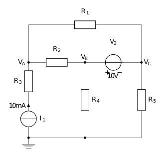
In Figure 1 we can see a circuit with two sources and we would like to know the voltage between $V_A$ and $V_B$. We cannot solve this circuit without the use of node-voltage or mesh current analysis. But here is the nice thing about superposition, we can verify that the circuit is linear (only resistors and sources here), so we can apply superposition.

Keeping the current source

We start by keeping our current source $I_1$. This means we have to convert our voltage source $V_1$ to a short circuit. The remaining circuit looks like this:

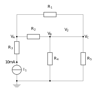
Superposition step 1 — Figure 2. The voltage source is converted to a short.

Now this is a circuit we can solve to figure out the voltage between $V_A$ and $V_B$. First we need to realize that $V_B$ and $V_C$ are now shorted together, so the same node. Next we can see that $R_4$ and $R_5$ are in parallel. With this information we can redraw the circuit to Figure 3.

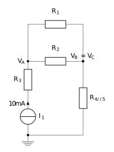
Superposition step 2 — Figure 3. Simplified circuit

The next step is to combine resistors $R_1$ and $R_2$ as they are also both parallel. We end up with Figure 4.

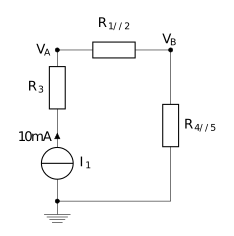
Superposition simplification step — Figure 4. Circuit simplified even further.

Now we have a simple circuit, with a known current, so we can easily calculate the voltage $V_{AB}$ with $V_{AB} = R_{1//2} \cdot I_1$

Keeping a voltage source

So we have solved part of a circuit, because now we need to solve it also for our other source, so this time we are going to remove the current source. Removing the current source means we have to convert it to an open circuit.

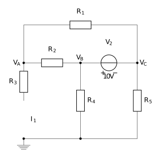
Superposition current source nulled — Figure 5. Superposition circuit with the current source removed.

Now we have a loose dangling resistor $R_3$. So we can just remove it.

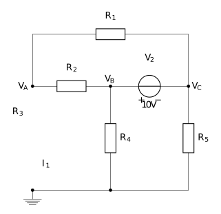
Now we can make a really big step, for the keen observer you can see that $R_1 + R_2$ is in parallel with $V_2$ which is in parallel with $R_4 + R_5$. With these sections being in parallel we can ignore the branch with $R_4$ and $R_5$. We can do this, as we are only interested in the voltage $V_{AB}$. For this voltage we only need the current through $R_2$ and the parallel circuit does not affect the current at all (you can check this yourself if you would like to). This leaves only with a very small circuit.

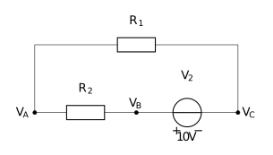
Superposition simplification — Figure 7. Fully reduced circuit

In this circuit we can solve for the voltage $V_AB$ either with Ohm’s law or with the voltage divider formula. With Ohm’s law we get:

$$ I_{ R_2} = \dfrac{V_2}{R_1 + R_2}$$

$$V_{AB} = -I_{R_2} \cdot R_2$$

Note that we have to use $-I_{R_2}$ because the current flow in this calculation is opposite to the result from the previous example. With the voltage divider we get: $$ V_{AB} = \dfrac{R_2}{R_1 + R_2} \cdot -V_2$$ Again the minus sign is required for the correct polarity.

Adding it all up

To get our final result we have to solve the circuit. First let’s choose $1k\Omega$ for all resistors. This allows us to calculate the result from our previous two solutions.

$$ V_{AB_current source} = R_{1//2} \cdot I_1 = 0.5k \cdot 10m = 5V$$

$$ V_{AB_voltage source} = \dfrac{R_2}{R_1 + R_2} \cdot -V_2 = \dfrac{1k}{2k} \cdot -10 = -5V$$

Summing it all up gives us 0 volt.

Checking the result

Let’s use node-voltage analysis to check if our result is correct. First we generate our set of equations:

$$ -10mA + \dfrac{V_A – V_B}{R_2} + \dfrac{V_A – V_C}{R_1} = 0$$

$$\dfrac{V_B-V_A}{R_2} + \dfrac{V_B – 0}{R_4} + \dfrac{V_C – 0}{R_5} + \dfrac{V_C – V_A}{R_1} = 0$$

$$V_B -V_C = 10$$

Did you notice that the current of $R_3$ is already known (due to the current source in series)? And did you also note the use of a super-node, because of the voltage source? If you did, you are getting the hang of node-voltage analysis! Now putting it all together in a matrix to get:

\begin{gather} \begin{bmatrix} \dfrac{1}{R_1}+\dfrac{1}{R_2} & \dfrac{-1}{R_2} & \dfrac{-1}{R_1}\\ \dfrac{-1}{R_1} +\dfrac{-1}{R_2} & \dfrac{1}{R_2}+\dfrac{1}{R_4} & \dfrac{1}{R_1}+\dfrac{1}{R_5} \\ 0 & 1 & -1 \\ \end{bmatrix} \begin{bmatrix} V_A \\ V_B \\ V_C \end{bmatrix} = \begin{bmatrix} 10m \\ 0 \\ 10 \\ \end{bmatrix} \end{gather}

If we compute the matrix with all values at $1k\Omega$ we get $V_A = 10V$, $V_B = 10V$ and $V_C = 0V$. So $V_{AB} = 0V$. Nice!

The ‘magic’ of disappearing sources

So you might be wandering why we can just remove the sources, and why voltage source become a short, and current source an open circuit. Well, we don’t really remove them, but we ‘dial them back to zero’ also called nulling.

What happens when we dial a voltage source to zero? The voltage across it get lower and lower up to the point where it reaches zero volts. Which circuit element also has zero volts of voltage drop? That’s right that is a wire, or a short circuit.

Similarly we can reduce the current of a current source. When it reaches zero it becomes a circuit element where no current can flow. In which element does no current flow at all? That is the open circuit, with no connection, no current.

This is the reason why we replace voltage sources with a wire (or short circuit) and current sources with and open circuit. It is also the reason why I prefer the European symbols for the voltage and current source. If you take away the circle around a voltage source you are left with a short circuit. If you take away the circle around a current source you end up with an open circuit. This so called impedance is reflected in the symbols and that is why I use them here on the site. And you can also you that as a neat trick to remember if a source was open or shorted (just remove the circle).

Recap

To solve a circuit with superposition we do four basic steps to get to the solution, these are:

First check if the circuit is linear, if yes, go to step 2, if no, use an other method to solve the circuit.
Null all sources except for one source and solve the circuit
Repeat step 2 for all sources in the circuit (so that you solve the circuit for each source once)
Add the results from each step together

This is superposition.